Tutorial 15: A loss network
A loss network models a system in which an arriving job (a call or connection) is admitted only if enough resources are free; otherwise it is blocked and lost rather than queued. Such models arise in circuit-switched telephony and in multirate broadband networks, where each class of call requires a fixed number of circuits on each link along its route.
In LINE a loss network is expressed as an open model whose stations sit inside a finite capacity region (FCR) with the DROP policy: when the region is full, arriving jobs are dropped. The stationary distribution is of product form, and the quantities of interest are the per-class blocking probabilities and the normalization constant g(C). Here two classes of calls share an infinite-server Delay station. Class 1 offers load 0.3 and class 2 offers 0.2 (arrival rate over service rate). The region admits at most 5 calls in total and at most 3 of each class.
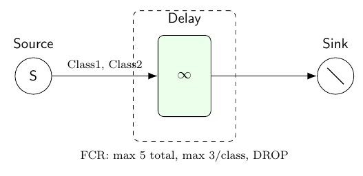
model = Network('LossNetwork');
% Block 1: nodes
source = Source(model, 'Source');
delay  = Delay(model, 'Delay');
sink   = Sink(model, 'Sink');
% Block 2: classes
class1 = OpenClass(model, 'Class1');
class2 = OpenClass(model, 'Class2');
source.setArrival(class1, Exp(0.3));
source.setArrival(class2, Exp(0.2));
delay.setService(class1, Exp(1.0));
delay.setService(class2, Exp(0.8));
% Block 3: topology
P = model.initRoutingMatrix();
P.set(class1, class1, source, delay, 1.0);
P.set(class1, class1, delay, sink, 1.0);
P.set(class2, class2, source, delay, 1.0);
P.set(class2, class2, delay, sink, 1.0);
model.link(P);
% Block 4: finite capacity region with dropping
fcr = model.addRegion({delay});
fcr.setGlobalMaxJobs(5);
fcr.setClassMaxJobs(class1, 3);
fcr.setClassMaxJobs(class2, 3);
fcr.setDropRule(class1, true);
fcr.setDropRule(class2, true);
% Block 5: solution
% Exact loss-network transform (lossn.exact), the default
AvgTable = SolverNC(model).avgTable()
% Monte Carlo summation (Ross-Wang): also estimates the normalizing constant
ncmci = SolverNC(model, 'method', 'mci', 'samples', 1e5, 'seed', 23000);
AvgTableMCI = ncmci.avgTable()
lG = ncmci.result.Prob.logNormConstAggr
% Simulation cross-check: LDES simulates the DROP region directly
AvgTableLDES = SolverLDES(model, 'seed', 23000, 'samples', 1e5).avgTable()Network model = new Network("LossNetwork");
// Block 1: nodes
Source source = new Source(model, "Source");
Delay delay = new Delay(model, "Delay");
Sink sink = new Sink(model, "Sink");
// Block 2: classes
OpenClass class1 = new OpenClass(model, "Class1", 0);
OpenClass class2 = new OpenClass(model, "Class2", 0);
source.setArrival(class1, new Exp(0.3));
source.setArrival(class2, new Exp(0.2));
delay.setService(class1, new Exp(1.0));
delay.setService(class2, new Exp(0.8));
// Block 3: topology
RoutingMatrix P = model.initRoutingMatrix();
P.set(class1, class1, source, delay, 1.0);
P.set(class1, class1, delay, sink, 1.0);
P.set(class2, class2, source, delay, 1.0);
P.set(class2, class2, delay, sink, 1.0);
model.link(P);
// Block 4: finite capacity region with dropping
model.addRegion(Collections.singletonList(delay));
Region fcr = model.getRegions().get(0);
fcr.setGlobalMaxJobs(5);
fcr.setClassMaxJobs(class1, 3);
fcr.setClassMaxJobs(class2, 3);
fcr.setDropRule(class1, true);
fcr.setDropRule(class2, true);
// Block 5: solution
// Exact loss-network transform (lossn.exact), the default
new SolverNC(model).avgTable().print();
// Monte Carlo summation (Ross-Wang): also estimates the normalizing constant
SolverNC ncMci = new SolverNC(model, "method", "mci");
ncMci.options.samples = 100000;
ncMci.options.seed = 23000;
ncMci.avgTable().print();
// Simulation cross-check: LDES simulates the DROP region directly
SolverLDES ldes = new SolverLDES(model, "seed", 23000);
ldes.options.samples = 100000;
ldes.avgTable().print();from line_solver import *
model = Network('LossNetwork')
# Block 1: nodes
source = Source(model, 'Source')
delay = Delay(model, 'Delay')
sink = Sink(model, 'Sink')
# Block 2: classes
class1 = OpenClass(model, 'Class1')
class2 = OpenClass(model, 'Class2')
source.set_arrival(class1, Exp(0.3))
source.set_arrival(class2, Exp(0.2))
delay.set_service(class1, Exp(1.0))
delay.set_service(class2, Exp(0.8))
# Block 3: topology
P = model.init_routing_matrix()
P.set(class1, class1, source, delay, 1.0)
P.set(class1, class1, delay, sink, 1.0)
P.set(class2, class2, source, delay, 1.0)
P.set(class2, class2, delay, sink, 1.0)
model.link(P)
# Block 4: finite capacity region with dropping
fcr = model.add_region(delay)
fcr.set_global_max_jobs(5)
fcr.set_class_max_jobs(class1, 3)
fcr.set_class_max_jobs(class2, 3)
fcr.set_drop_rule(class1, True)
fcr.set_drop_rule(class2, True)
# Block 5: solution
# Exact loss-network transform (lossn.exact), the default
print(SolverNC(model).avg_table())
# Monte Carlo summation (Ross-Wang): also estimates the normalizing constant
print(SolverNC(model, method='mci', samples=100000, seed=23000).avg_table())
# Simulation cross-check: LDES simulates the DROP region directly
print(SolverLDES(model, seed=23000, samples=100000).avg_table())#include "line/solvers/nc/solver_nc_runner.h"
#include "line/solvers/wrappers/ldes/solver_ldes.h"
Network model("LossNetwork");
Source source(model, "Source");
Delay delay(model, "Delay");
Sink sink(model, "Sink");
OpenClass class1(model, "Class1");
OpenClass class2(model, "Class2");
source.set_arrival(class1, Exp(0.3));
source.set_arrival(class2, Exp(0.2));
delay.set_service(class1, Exp(1.0));
delay.set_service(class2, Exp(0.8));
Routing P;
P.set(class1, class1, source, delay, 1.0);
P.set(class1, class1, delay, sink, 1.0);
P.set(class2, class2, source, delay, 1.0);
P.set(class2, class2, delay, sink, 1.0);
model.link(P);
model.add_region(std::vector<std::size_t>{delay},
std::vector<double>{3.0, 3.0},
5.0,
std::vector<DropStrategy>{DropStrategy::DROP,
DropStrategy::DROP});
nc::NcSolverOptions exactOptions;
const mva::AvgResult<double> exact =
nc::solver_nc_run_analyzer(model.get_struct(), exactOptions);
nc::NcSolverOptions mciOptions;
mciOptions.method = "mci";
mciOptions.samples = 100000;
const mva::AvgResult<double> monteCarlo =
nc::solver_nc_run_analyzer(model.get_struct(), mciOptions);
// Simulation cross-check: LDES simulates the DROP region directly
ldes::LdesOptions simOptions;
simOptions.seed = 23000;
simOptions.samples = 100000;
const ldes::LdesResult simulated =
ldes::solver_ldes(model.get_struct(), simOptions);Expected Output
SolverNC recognizes the single-Delay DROP region as a loss network and offers two methods: the default exact loss-network transform and the Monte Carlo summation (Ross-Wang), which also estimates the log-normalization constant log g(C). All three solutions agree closely, confirming the product-form result against simulation:
AvgTable =                          % SolverNC, lossn.exact (default)
    Station    JobClass     QLen       Util      RespT    ResidT     ArvR       Tput
     Delay      Class1     0.29898    0.29898       1         1     0.29898    0.29898
     Delay      Class2     0.24947    0.24947    1.25      1.25     0.19958    0.19958
AvgTableMCI =                       % SolverNC, mci (Ross-Wang)
     Delay      Class1      0.299      0.299       1         1      0.299      0.299
     Delay      Class2     0.2495     0.2495     1.25      1.25     0.1996     0.1996
lG = 0.5494                         % log-normalization constant log g(C)
AvgTableLDES =                      % SolverLDES simulation
     Delay      Class1     0.29825    0.29932    0.99645    0.99645    0.29961    0.29932
     Delay      Class2     0.24917      0.249     1.2506     1.2506    0.19941     0.1992