Tutorial 14: Open Cluster
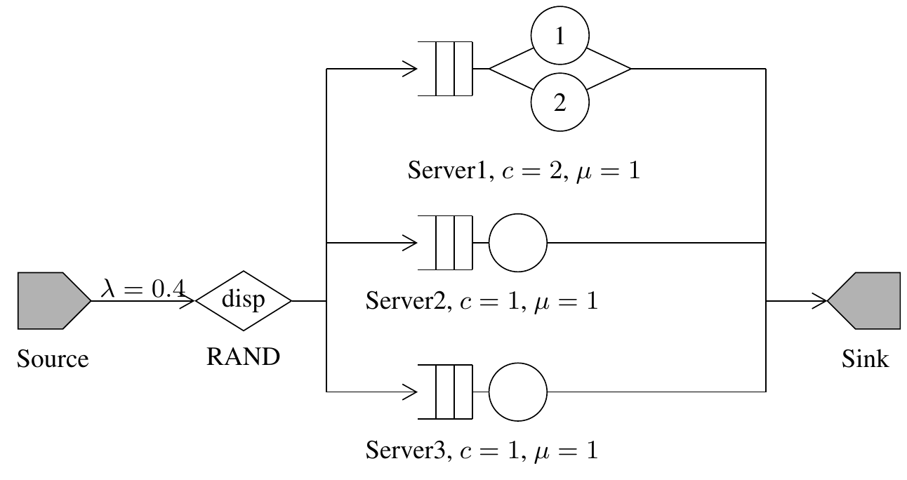
We model an open cluster: a single open class of jobs flows from a Source through a Router (the dispatcher) into one of M=3 parallel processor-sharing servers, after which it leaves the system through a Sink. We illustrate two equivalent ways of building this model: a one-liner factory (Network.clusterPs), and the more flexible Cluster builder, which we use to compare two dispatching policies on the same cluster.
Block 1: One-liner factory
We start with the one-liner factory. The arrival rate is λ = 0.4 and each server has a mean service time of D = 1, giving a per-server utilization of λ/M ≈ 0.133 under random dispatching.
lambda = 0.4;
D = ones(3,1);
model = Network.clusterPs(lambda, D, RoutingStrategy.RAND);
avgTable = MVA(model).getAvgTable()Matrix lambda = new Matrix("[0.4]");
Matrix D = new Matrix("[1.0; 1.0; 1.0]");
Network model = Network.clusterPs(lambda, D, RoutingStrategy.RAND);
new MVA(model).getAvgTable().print();from line_solver import *
lam = [0.4]
D = [[1.0], [1.0], [1.0]]
model = Network.cluster_ps(lam, D, RoutingStrategy.RAND)
print(MVA(model).get_avg_table())// Network::cluster_ps is not part of the C++ port. Build the equivalent
// Source -> three queues -> Sink network explicitly, as in Block 2 below.Expected MVA output (traffic split evenly across the three servers)
    Station    JobClass     QLen       Util      RespT     ResidT      ArvR       Tput
    _______    ________    _______    _______    ______    _______    _______    _______
    Source      Class1           0          0         0          0          0        0.4
    Server1     Class1     0.15263    0.13333    1.1448    0.38158    0.13333    0.13333
    Server2     Class1     0.15263    0.13333    1.1448    0.38158    0.13333    0.13333
    Server3     Class1     0.15263    0.13333    1.1448    0.38158    0.13333    0.13333
Block 2: Cluster builder with multi-server queues
We now switch to the chainable Cluster builder to introduce non-uniform multi-server queues, replacing PS with FCFS and giving Server 1 two parallel cores (M/M/2, the others stay M/M/1):
cluster = Cluster().setNumStations(3).setArrivalRate(0.4).setServiceRate(1.0);
cluster.setScheduling(SchedStrategy.FCFS);
cluster.setStationServers([2; 1; 1]);   % Server1 = M/M/2, Server2/3 = M/M/1
avgTableFcfs = MVA(cluster.build()).getAvgTable()Cluster cluster = new Cluster().setNumStations(3).setArrivalRate(0.4).setServiceRate(1.0)
.setScheduling(SchedStrategy.FCFS)
.setStationServers(new int[] {2, 1, 1});
new MVA(cluster.build()).getAvgTable().print();cluster = (Cluster().set_num_stations(3).set_arrival_rate(0.4).set_service_rate(1.0)
.set_scheduling(SchedStrategy.FCFS)
.set_station_servers([2, 1, 1]))
print(MVA(cluster.build()).get_avg_table())Network model("Cluster");
Source source(model, "Source");
Sink sink(model, "Sink");
OpenClass cls(model, "Class1");
source.set_arrival(cls, Exp(0.4));
const std::vector<double> servers{2, 1, 1};
Routing P;
std::vector<std::size_t> queues(servers.size());
for (std::size_t i = 0; i < servers.size(); ++i) {
queues[i] = model.add_queue(
"Server" + std::to_string(i + 1), SchedStrategy::FCFS);
model.set_number_of_servers(queues[i], servers[i]);
model.set_service(queues[i], cls, Exp(1.0));
P.set(source, queues[i], 1.0 / double(servers.size()));
P.set(queues[i], sink, 1.0);
}
model.link(P);Block 3: Cross-check LDES and SSA on the FCFS cluster
We then cross-check the same FCFS cluster under two simulators. LDES is LINE's discrete-event simulator built on the SSJ library, invoked as a subprocess; SSA is LINE's native next-reaction-method stochastic simulator. Both produce statistically equivalent results on this open-class cluster and exercise the multi-server FCFS path.
disp(LDES(cluster.build(), 'seed', 23000, 'samples', 20000).getAvgTable());
disp(SSA(cluster.build(), 'seed', 23000, 'samples', 20000).getAvgTable());new LDES(cluster.build(), "seed", 23000, "samples", 20000).getAvgTable().print();
new SSA(cluster.build(), "seed", 23000, "samples", 20000).getAvgTable().print();print(LDES(cluster.build(), seed=23000, samples=20000).get_avg_table())
print(SSA(cluster.build(), seed=23000, samples=20000).get_avg_table())#include "line/solvers/ssa/ssa_dispatch.h"
#include "line/solvers/wrappers/ldes/solver_ldes.h"
ldes::LdesOptions ldesOptions;
ldesOptions.seed = 23000;
ldesOptions.samples = 20000;
const ldes::LdesResult ldesResult =
ldes::solver_ldes(model.get_struct(), ldesOptions);
ssa::SsaOptions options;
options.seed = 23000;
options.samples = 20000;
const ssa::SsaSolution result =
ssa::solver_ssa(model.get_struct(), options);Block 4: Compare dispatching policies
Finally, we compare random and round-robin dispatching on a uniform PS cluster. Round-robin is non-product-form, so we drop to LDES with a small sample budget. The compareDispatching helper runs the same cluster under each policy and returns one result table per policy.
cluster2 = Cluster().setNumStations(3).setArrivalRate(0.4).setServiceRate(1.0);
cluster2.setScheduling(SchedStrategy.PS);
solverFcn = @(m) LDES(m, 'seed', 23000, 'samples', 5000).getAvgTable();
results = cluster2.compareDispatching(solverFcn, ...
    [RoutingStrategy.RAND, RoutingStrategy.RROBIN]);

keys_ = results.keys;
for k = 1:numel(keys_)
    fprintf('\n=== Dispatching: %s ===\n', keys_{k});
    disp(results(keys_{k}));
endCluster cluster2 = new Cluster().setNumStations(3).setArrivalRate(0.4).setServiceRate(1.0)
.setScheduling(SchedStrategy.PS);
Function<Network, NetworkAvgTable> solverFcn =
m -> new LDES(m, "seed", 23000, "samples", 5000).getAvgTable();
cluster2.compareDispatching(solverFcn,
RoutingStrategy.RAND, RoutingStrategy.RROBIN)
.forEach((policy, table) -> {
System.out.println("=== Dispatching: " + policy + " ===");
table.print();
});cluster2 = (Cluster().set_num_stations(3).set_arrival_rate(0.4).set_service_rate(1.0)
.set_scheduling(SchedStrategy.PS))
solver_fcn = lambda m: LDES(m, seed=23000, samples=5000).get_avg_table()
for policy in (RoutingStrategy.RAND, RoutingStrategy.RROBIN):
cluster2.set_dispatching(policy)
print(f"=== Dispatching: {policy} ===")
print(solver_fcn(cluster2.build()))// On a uniform cluster with an explicit dispatcher Router:
for (const RoutingStrategy policy :
{RoutingStrategy::RAND, RoutingStrategy::RROBIN}) {
model.set_routing(dispatcher, cls, policy);
ldes::LdesOptions options;
options.seed = 23000;
options.samples = 5000;
const ldes::LdesResult result =
ldes::solver_ldes(model.get_struct(), options);
}For this lightly loaded cluster both policies produce very similar response times; differences become visible only at higher utilization, where round-robin reduces variability across servers compared with the i.i.d. split produced by random dispatching.