Tutorial 7: Delayed-hit caches with a retrieval system
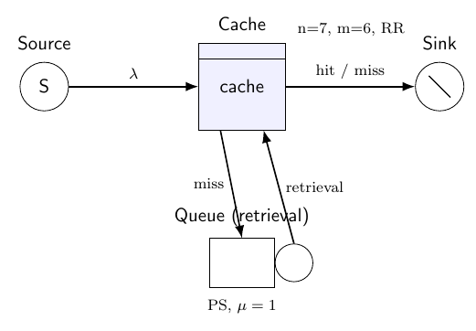
In a delayed-hit cache a miss does not complete instantaneously: the requested item must be fetched through a retrieval system, a small network of queues that models the cost of retrieving the item. While an item is being fetched, further requests for the same item become delayed hits: they wait for the in-flight fetch to complete rather than triggering a new retrieval.
LINE represents the retrieval system with setRetrievalSystem and analyses it exactly with NC (a product-form recurrence) and approximately, including the expected latency, with MVA (a fixed-point heuristic). This example uses n=7 items, a single cache list of capacity m=6 under random replacement (RR), and a single processor-sharing (PS) retrieval station of unit service rate. Requests arrive in a Poisson stream and read items with the popularity vector (49,49,49,49,7,1,1)/205. On a miss, the read request switches to a retrieval class routed through the retrieval queue and back to the cache; setRetrievalSystem installs the cache to queue to cache routing automatically.
accessProb   = [49, 49, 49, 49, 7, 1, 1] / 205;   % item popularities
serviceRates = ones(1, 7);                         % per-item fetch rates (mu=1)
n = numel(serviceRates);

model     = Network('Retrieval');
source    = Source(model, 'Source');
cacheNode = Cache(model, 'Cache', n, [6], ReplacementStrategy.RR);
queue     = Queue(model, 'Queue', SchedStrategy.PS);   % retrieval station
sink      = Sink(model, 'Sink');

jobClass  = OpenClass(model, 'InitClass', 0);
hitClass  = OpenClass(model, 'HitClass', 0);
missClass = OpenClass(model, 'MissClass', 0);

source.setArrival(jobClass, Exp(1));
cacheNode.setRead(jobClass, DiscreteSampler(accessProb));
cacheNode.setHitClass(jobClass, hitClass);
cacheNode.setMissClass(jobClass, missClass);
queue.setService(jobClass, Exp(1));   % retrieval service is taken from the read class
cacheNode.setRetrievalSystem(jobClass, missClass, queue);

P = model.initRoutingMatrix();
P{jobClass, jobClass}(source, cacheNode) = 1;
P{hitClass, hitClass}(cacheNode, sink)   = 1;
P{missClass, missClass}(cacheNode, sink) = 1;
model.link(P);

% Exact analysis (NC): product-form recurrence
NC(model).getAvgTable;
hit  = cacheNode.getHitRatio;     % 0.982722  (exact)
miss = cacheNode.getMissRatio;    % 0.015118  (delayed = 1 - hit - miss = 0.002160)

% Approximate analysis (MVA): fixed-point heuristic, returns latency
MVA(model).getAvgTable;
hit    = cacheNode.getHitRatio;   % 0.975727  (FPI)
residt = cacheNode.getResidT; % 1.015496double s = 205;
double[] accessProb = {49/s, 49/s, 49/s, 49/s, 7/s, 1/s, 1/s}; // item popularities
double[] serviceRates = {1, 1, 1, 1, 1, 1, 1}; // per-item fetch rates
int n = serviceRates.length;
Network model = new Network("Retrieval");
Source source = new Source(model, "Source");
Cache cacheNode = new Cache(model, "Cache", n, new Matrix(new double[][]{{6}}), ReplacementStrategy.RR);
Queue queue = new Queue(model, "Queue", SchedStrategy.PS); // retrieval station
Sink sink = new Sink(model, "Sink");
OpenClass jobClass = new OpenClass(model, "InitClass", 0);
OpenClass hitClass = new OpenClass(model, "HitClass", 0);
OpenClass missClass = new OpenClass(model, "MissClass", 0);
source.setArrival(jobClass, new Exp(1));
cacheNode.setRead(jobClass, new DiscreteSampler(new Matrix(new double[][]{accessProb})));
cacheNode.setHitClass(jobClass, hitClass);
cacheNode.setMissClass(jobClass, missClass);
queue.setService(jobClass, new Exp(1)); // retrieval service is taken from the read class
cacheNode.setRetrievalSystem(jobClass, missClass, queue);
RoutingMatrix P = model.initRoutingMatrix();
P.set(jobClass, jobClass, source, cacheNode, 1.0);
P.set(hitClass, hitClass, cacheNode, sink, 1.0);
P.set(missClass, missClass, cacheNode, sink, 1.0);
model.link(P);
// Exact analysis (NC)
new NC(model).getAvgTable();
Matrix hit = cacheNode.getHitRatio(); // 0.982722 (exact)
Matrix miss = cacheNode.getMissRatio(); // 0.015118
// Approximate analysis (MVA): returns latency
new MVA(model).getAvgTable();
Matrix hitFpi = cacheNode.getHitRatio(); // 0.975727 (FPI)
Matrix residt = cacheNode.getResidT(); // 1.015496val s = 205.0
val accessProb = doubleArrayOf(49/s, 49/s, 49/s, 49/s, 7/s, 1/s, 1/s)
val serviceRates = doubleArrayOf(1.0, 1.0, 1.0, 1.0, 1.0, 1.0, 1.0)
val n = serviceRates.size
val model = Network("Retrieval")
val source = Source(model, "Source")
val cacheNode = Cache(model, "Cache", n, Matrix(arrayOf(doubleArrayOf(6.0))), ReplacementStrategy.RR)
val queue = Queue(model, "Queue", SchedStrategy.PS) // retrieval station
val sink = Sink(model, "Sink")
val jobClass = OpenClass(model, "InitClass", 0)
val hitClass = OpenClass(model, "HitClass", 0)
val missClass = OpenClass(model, "MissClass", 0)
source.setArrival(jobClass, Exp(1.0))
cacheNode.setRead(jobClass, DiscreteSampler(Matrix(arrayOf(accessProb))))
cacheNode.setHitClass(jobClass, hitClass)
cacheNode.setMissClass(jobClass, missClass)
queue.setService(jobClass, Exp(1.0)) // retrieval service is taken from the read class
cacheNode.setRetrievalSystem(jobClass, missClass, queue)
val P = model.initRoutingMatrix()
P.set(jobClass, jobClass, source, cacheNode, 1.0)
P.set(hitClass, hitClass, cacheNode, sink, 1.0)
P.set(missClass, missClass, cacheNode, sink, 1.0)
model.link(P)
NC(model).getAvgTable()
val hit = cacheNode.getHitRatio() // 0.982722 (exact)
val miss = cacheNode.getMissRatio() // 0.015118
MVA(model).getAvgTable()
val hitFpi = cacheNode.getHitRatio() // 0.975727 (FPI)
val residt = cacheNode.getResidT() // 1.015496from line_solver import *
import numpy as np
access_prob = list(np.array([49, 49, 49, 49, 7, 1, 1]) / 205) # item popularities
service_rates = [1.0] * 7 # per-item fetch rates
n = len(service_rates)
model = Network('Retrieval')
source = Source(model, 'Source')
cache_node = Cache(model, 'Cache', n, [6], ReplacementStrategy.RR)
queue = Queue(model, 'Queue', SchedStrategy.PS) # retrieval station
sink = Sink(model, 'Sink')
job_class = OpenClass(model, 'InitClass', 0)
hit_class = OpenClass(model, 'HitClass', 0)
miss_class = OpenClass(model, 'MissClass', 0)
source.set_arrival(job_class, Exp(1))
cache_node.set_read(job_class, DiscreteSampler(access_prob))
cache_node.set_hit_class(job_class, hit_class)
cache_node.set_miss_class(job_class, miss_class)
queue.set_service(job_class, Exp(1)) # retrieval service is taken from the read class
cache_node.set_retrieval_system(job_class, miss_class, queue)
P = model.init_routing_matrix()
P.set(job_class, job_class, source, cache_node, 1.0)
P.set(hit_class, hit_class, cache_node, sink, 1.0)
P.set(miss_class, miss_class, cache_node, sink, 1.0)
model.link(P)
# Exact analysis (NC)
NC(model).get_avg_table()
hit = cache_node.get_hit_ratio() # 0.982722 (exact)
miss = cache_node.get_miss_ratio() # 0.015118
# Approximate analysis (MVA): returns latency
MVA(model).get_avg_table()
hit = cache_node.get_hit_ratio() # 0.975727 (FPI)
residt = cache_node.get_residt() # 1.015496Expected Output
NC detects the retrieval system and applies the exact product-form recurrence, returning the hit and miss probabilities of the read class; the delayed-hit probability is the residual 1 - hit - miss. MVA uses the fixed-point heuristic and additionally returns the expected retrieval latency Z (the mean delay incurred by misses and delayed hits), which the exact (NC) and simulation (CTMC, SSA) solvers leave unset (NaN).
NC  (exact):  hit = 0.982722   miss = 0.015118   delayed = 0.002160
MVA (FPI):    hit = 0.975727   residT = 1.015496  (retrieval latency)
The retrieval system may contain infinite-server (IS) stations and single-server stations with PS, SIRO, FCFS or LCFS-PR scheduling. The discrete-event simulator LDES also simulates delayed-hit caches and measures the retrieval latency directly, providing a cross-check for the analytical solvers.